System Dynamics Lecture Notes 2007-05

These are my lecture notes of the 5. session of IE 602 System Dynamics Analysis and Design course in Industrial Engineering Graduate Program of Bogazici University. You can find the video of the lecture in Google Videos. The course is given by Prof. Yaman Barlas.


Lecture Video Part I
Lecture Video Part II
Lecture Video Part III

Figures are here: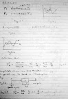



Tools for Sensitivity Analysis

1. Analytical sensitivity
2. By simulation experiment
One value at a time approach. You take each parameter in high low middle levels. Then leave it at middle. Do this with other parameters. If you have p parameters then you will do 3p experiments. The simplest approach.
3. Experiment design: Systematic way of carrying out experiment in simulations.
3.1
People say you need to change each parameter to each parameter level in all levels. This is full factorial design under experiment design. You have l^p runs. This assumes that there is no errors due to randomization. You have to experiment each data 3-4 repeatedly for stat estimation. Then it becomes an impossible problem. You use this in very small models. Or If you want to analyze only 5-6 parameters.
3.2. Fractional factorial design. Under certain assumptions you can get a good idea about the shape of response function of the experiment by not carrying out full factorial experiment but by fraction of it. Maybe by only 10%. It eliminates all... The simplest interaction term is two term inter. Higher terms very high number of experiment. If you have 10 variables, you can at most design two term or triple experiments. The design is called fractional factorial design. You make certain assumptions either high term inter don't exist. or they can be neglected. Or you know results that you obtain are tentative. Then you have a sample based on these assumptions. This is the starting point in your work.
3.4. Random sampling. Another reduction approach. Assume that full factorial experiment has hundred thousand required experiments. Then you take some random numbers and pick some of the experiments. This assumes you don't have any idea of the shape of the function. Because if you know the shape then you don't do totally random sampling. Now representativeness is important. It is rarely used.
3.5. Latin hypercube sampling. More advanced approach. Some sort of stratified sense. It is random but not purely. Each parameter rage is divided into N strata. That is they have N different values. For each parameter you randomly pick one value. One run is one random values for each parameter. Fig.5.1. You do this without replacement. You never want to try the same combination again. Next time you obtain another comb of parameter values. You repeat this N times. Number of values you tried. Full sensitivity of each parameter is focus. Focus is on if you have on parameter you have full detail of high resolution of this parameter. Since you do this without replacement, it assumes that all parameter effects are independent. This is quite restrictive. The adv is it provides with few experiments very homogeneous coverage of experiment space.
3.3. Taguchi design. Modern approach. Very practical design. It's a special quite reduced form of fractional factorial design.18 predefined tables are designed to fit most commons situations. A simple cookbook approach. Huge reduction of number of experiments. Assumption is most interactions are nonexistent. Few selected some two level interactions can be modeled. In all designs all higher order interactions are nonexistent. It assumes further parameter output relation is assumed linear.
Let's say the Output measure is amplitude. Fig.5.2. Question: How sensitivity is amplitude to ordering period. The assumption is Fig.5.3. This is not the model. This comes as a result of the solution of the model.
Fig.5.4. If inventory is equal to some K plus A time something. This is the solution of the model let's assume. A is amplitude of this oscillatory function. Taguchi design says A is a linear function of some parameter. Model can be nonlinear.
I think this is not a very safe assumption.
Q: Higher order inter are nonexistent, is assumed. Doesn't it contradict systemic approach. It tries to reveal inter effects.
A: In general this is true.We are building systemic models to discover simultaneous effects of multiples measures. But quantitatively changing values of parameters you cannot extract out the sensitivity of the output by increasing it values at different levels and by not simultaneous changing other levels. I am not sure the statements are equal. If model is linear, the two statements are equal.

Guidelines for sensitivity analysis:
We need to use our knowledge of the model to reduce number of experiment.
1. Seek behavior pattern sensitivity rather than numeric sensitivity. Don't spend months on numerical sensitivity of the amplitude in Fig.5.2. For example in Fig 5.4 seek the sensitivity that causes a to turn into b. From growing oscillation to damping oscillation.
2. Positive feedback loops have in general more influence such strong behavior pattern sensitivity of the model. They are destabilizing loops. They are crash or growth lops.
3. Range of parameter values that you try out. When you do sensitivity analysis especially for parameter estimation and policy analysis. Restrict parameter set to a realistic set of parameters. But you can do this for validity testing.
4. You may have some parameters estimated using stat tools. On these parameters you don't need extensive sensitivity testing if they are not decision parameters.
5. When multiple parameters are simultaneous altered, you know that in real life it is inconsistent that death rate is much higher and birth rate is much lower. When death rate goes up birth rate goes also up.Not for validity testing.

Mathematical equations:
To show you idea of feedback sensitivity.
Mathematical Sensitivity Analysis
Definition: Sensitivity of S^M_K M:output measure, K:parameter.
Equation 5.5
If you find M=f(k) you need have derived the solution. You can not find solution in general in dynamical systems.
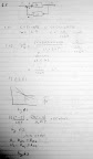
e.g.. A linear (feedback) dynamical system. In block notation: Fig.5.6.
What transfer function does is it multiplies r and obtains C.
G: Transfer function in frequency (s) domain. Then C=r G. Here C would be in s. First you take Laplace trans to obtain G.
This Fig.5.6 called open system.
Sensitivity of output C wrt G. S_G^C. Equation 5.7
This is clear because of C=rG.
Now consider adding a feedback loop.
Fig.5.8
You observe output and do something. These inputs and outputs are not flows. G is not derivative of flows. This has integrations in itself, but it is block diagram and just means C=rG.
When you have two lines entering into a block, you take plus and minus, that is the difference. e.g. you take an action based on difference of desired inventory and measured inventory.
Mathematically 5.9 C=(r-b)G
b=cH
C=(r-cH)G...
So combined block is 5.9.a
5.10
This is 5.10.a is sensitivity of percent change in C to G. The higher H, the lower sensitivity, in general. It is not anymore a constant sensitivity like 5.7.a.
Reduced sensitivity of negative feedback control system.