26 February 2007 Structure Validity - Verification Differences Methodology to indirect structure testing software: In general, you can't examine the output and deduce the structure from the behavior. This is general fact. But logically, write the expected behavior under extreme conditions. Mantıksal tahminlerle, aşırı durumlarda, sonuçtan çıkarak yapıyı tahmin edebilirsin. There is first of all a base behavior. Fig. 2.1 In condition c, we expect some other behavior pattern, which is different than base behavior. Fig.2.2 But there is a subjective part as well. If the behavior is a little different like Fig.2.3 is this acceptable? SIS Software: 1. Teach the template of dynamical patterns. Program should recognize the patterns. E.g. Decline: subclasses: can go to zero or not Growth and decline: subclasses: not S shaped growth, but a goal seeking growth. There are about twenty patterns to categorize all the fundamental patterns. Pattern recognition: Complicated pattern recognition algorithms are about faces, handwriting. But they are not fit for functions. They don't exploit the properties of functions. Any function is a succession of curves. With two derivatives and ranges on these, we can summarize dynamical pattern of slopes and curvatures. For example, a curve might have such ranges: In the first range first derivative is positive, second is negative, then an inflection point. And so on. States are characterized by these two components (first derivative and second derivative). Then you can characterize both derivatives being negative, second zero, first positive so forth. So a pattern like Fig.2.2 can be summarized by a few successions of states. We have some more measures: Constants: are they zero or more? Then you give hundreds of noisy data of each class. E.g. for Fig.2.2 the bunch in Fig. 2.4 are training data. They all belong to overshoot and decay to zero class. Computer brings some sort of probability matrix of the state transitions. Then it produces transition probability matrix. Then it saves them. So, it averages all these. Then stamps class transition probability matrix. This is sort of signature of this class. You give some noise for patterns, for example you can add one more transient growth before the expected decay. It should probabilistically distinguish the data that looks like some pattern and determine to which class the data is closest? The likelihood to belonging to a class is maximized for one of the classes. Fig. 2.5 The algorithm is explained in thesis or working paper. Example just to prove it works. Base behavior of a model: Change the parameters and obtain n output. Fig. 2.6 what is the new pattern? Algorithm says new pattern: negative exponential growth. Parameter Calibration Fig.2.7 For example, the aim is to change the growth to an s-shaped growth from exponential growth. Is this possible? Gönenç bu konuda çalışıyor. It runs all the combinations of parameters. But these combinatorial run becomes too many. Then it says best parameters. Bu araştırma konusu çok yüksek getiri sağlıyor. Bu arama işlemi, akılılaştırılabilir mi (intelligence)? Gönenç çalışıyor. Heat algorithm, genetic algorithms heal climbing. They depend on problem instances. Eğer çok sayıda yapıda çalışan algoritma bulabilirsek, bu araştırma olur. Tek bir yapıda değil. Modellerin benzerliğinden kasıt: modelin yapısı. Bu aslında matematiksel fonksiyonun biçmidir. Calibration with input data: SIS: Bu konuda ödevler verilecek. Behavior Validity It focuses on patterns, but not like pattern classification problem. It is qualitative. BV is quantitative validation. Real system is oscillations class, is my model behavior oscillatory? This is not the subject of behavior validity. Fundamental behavior is oscillatory. Then compare the patterns. What are pattern components of oscillations? Fig.2.8. Trend, period, amplitude. More measures? Phase angle? That is how it starts? Önce inişe mi geçiyor, çıkışa mı? For many patterns it is like Fig. 2.9 (overshoot and decay). What components? Max, equilibrium, time points, slopes Dynamics of any system can be stated in two parts: transient, steady states. Fig.2.10a. Any dynamical system has these. Transient is caused by initial disequilibrium of system. After initial disequilibrium goes away, what the system does is steady state. This has no dynamics in Fig.2.10a. Whereas in b steady state behavior is damping oscillation. There is a big difference between two. You can apply this to every pattern. You can even have very strange dynamics like in Fig. 2.11. In steady state, there is a succession of boom and bust. Then equilibrium, then again boom and bust happens. Steady state is a succession of overshoot and equilibrium. Fundamental difference between these two: a) There is a steady state and transient state b) There is only transient Statistical estimation cannot be applied to transient behavior. There is no repeated data thus you can’t obtain x bar i.e. average. You have to have repeated date. You can statistically compute the period of 2.10b. In Fig. 2.11You can statistically compute period but not maximum. In 2.10a, there is a single pint. For that reason transient behavior is not analyzed by statistical estimators. This is life cycle problem. A business collapses. Another example is some goal seeking control problem, thermostat. It just arrives to a constant temperature. They don’t have repetitive data. Behavior Validity Testing Software: BTS II First question: is it transient dynamics? Then you forget statistical estimations. You just find graphical measurements: maxima, minima, inflection points, and distances. In steady state there are more statistical measures: like trend regression, smoothing. First thing, to do: detrend (remove trend) the data. If any time pattern has trend in it, most of statistical measure, like variance, mean, autocorrelation functions are impossible to estimate. Most stat measures are related to x bar. If x bar doesn't exist, then you don have them. Is there a trend? If there is, estimate trend and remove trend. (Trend regression) Then you do smoothing. This is for real data. In model, you turn off noisy parameters. Fig.2.12. It looks like oscillatory behavior. First smooth this by filtering like moving averages, exponential smoothing. Rest is standard tools. Multi-step procedure: Barlas has ready packages for statistical measures. Otomatik olarak islemleri yapiyor. Autocorrelation: Estimate autocorrelation function, they are like signatures of dynamical patterns. How successive data points are related. 0: 1. How 1 is correlated to 0 point. Fascinating is it doesn’t only show short term autocorrelation of model. Kısa dönemli korelasyonla, uzun dönemli korelasyon farklı. AC data has periodic behavior. At 22 is the peak again. That is not coincidence. This 22 is the estimate of noisy oscillatory time series. If time series is periodic, autocorrelation is periodic with the same period. Take difference between two autocorrelation functions. Find 95% confidence band. Difference lies out of the band. Then you reject the hypothesis. Spectral density function is transformation of ac function in frequency domain. Fourier transformations of ac function in s domain. Spectral density function use windowing technique. To exaggerate peaks. It is stat estimation technique. This ay spectral density function will show peaks frequencies at which time series has max energy content. It is also called power spectrum. Power content of time series is maximal at what time points? This will peak at dominating frequencies. Max occurs again at 20. Cross correlation: It is a measure that (ac was how in a given time series successions. time points are correlated?) cc is good old correlation function. How x and y are correlated? Take two data sets as x and y. You cross multiply x and y. Then divide by standard dev. That is Pearson correlation function. If it is positive, then data are positively correlated like lung cancer and cigarette smoking. CC is a generalization of that. I give you x and y. Cross correlate by different lengths x1 time y2. CC is a function of lag; only at lag 0 is good old correlation. Function is to find at any lag the cc of x and y. (Slayt PPde) If at 0 the peak: then they are at perfect phase. When out of phase, peak somewhere else. Amplitude: Compare discrepancy coefficient. Single measure that summarizes overall numeric fit. Next time I will show formulas. Compare trend in amplitude:
Figures are here: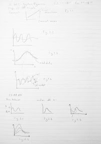

skip to main |
skip to sidebar
My daily weblog... Subjects: - Engineering and design - Methods for quality software development - Java platform - System dynamics - Knowledge management - My personal ideas...
Google Reader Sharings
About Me

Labels
- system-dynamics (6)
- validity (3)
- internet (1)
- lean-thinking (1)
- productivity (1)
Blog Archive
-
▼
2007
(7)
-
▼
March
(6)
- IE 602 System Dynamics Lecture Notes 2007-01 - By ...
- System Dynamics Lecture Notes 2007-05
- IE 602 System Dynamics Lecture Notes 2007-04 - By ...
- IE 602 System Dynamics Lecture Notes 2007-03 - By ...
- IE 602 System Dynamics Lecture Notes 2007-02 - By ...
- IE 602 System Dynamics Lecture Notes 2007-01 - By ...
-
▼
March
(6)