01 March 2007 20070301 BTS (Behavior Testing Software) Tools in BTS Slayt grafikler Assume that a certain system has these types of behavior. Fig.3.1 First graph (model generative) has near perfect fit. Second: error: trend. Since there is a trend error, means differ. Thus ac function can’t be found. Third: period error. Can you discuss phase angles? They will be periodically in or out of phase. Fourth: First has almost non-modellable noise. Fourth noise is questionable. Modellable smaller period noise. Autocorrelation function or spectral density function will reveal this smaller oscillation. Variance of real data will be larger. Fifth: out of phase. Cross correlation function will give a maximum at a certain lag. It can give a lag error but it will be random like 1. Sixth: mean error Seventh: amplitude error First you need detrend the data. Then do smoothing. Then check the periods. Until you remove period error. Then check phases and so on. So there is a logical order of tests. Trend removal: Models can be linear, quadratic, and exponential. Take cross products and take the average. That is covariance function. Then there is notion of lag. If there is no lag, then it is covariance. If no lag, covariances in the data that are one lag apart. k can be at most 1/5 of the data. Covariance is a number it can be positive or negative. If large then there is a large covariance negative or pos. But how large is large? You normalize it. To normalize it, you divide it by max possible covariance. Max possible covariance is at zero, this is actually variance. This is famous autocorrelation function. By definition it is less than one. Any value which is statistically significantly larger than zero means, there is a significant covariance at lag k. One specific usage is to estimate the period of data. You can also prove that, if periodicity is t, autocorrelation function has period of t. That way time series is very noisy, autocorrelation function will be noise free. Another useful usage: general comparison of autocorrelation structures between real data and model generated data. AC is signature of data. AC is hard to.. Higher order sophisticated smaller movements in real data are captured by model itself? Ac structure of data and ac function of model. This is signature. Rather than comparing g real data and model generated output one by one. If you do that, you get huge errors. Then compare their signatures i.e. autocorrelation functions. Do the ac functions differ at any lag significantly? Each ac function is a statistic. Using variance of ac function, you construct confidence band or control limits. H0: All r (variance sanirim) are equal. At all lags. It is all multi ... test. It is hard to estimate alpha value of function, because it is not a single test. If you reject, only one is ejected. It is hard problem. They are not independent. If you reject at lag 2, you may also reject at lag 3. They are not independent hypothesis, they are auto correlated too. Alphas are not clear, but test is okay. Estimating spectral density function: It is Fourier transformation of ac function. It is a function of time. That is it is in time domain. You transform it to obtain a function in frequency domain. S is frequency. SD function details won't be discussed. You transform ac. Then use windowing (filtering) technique. Then you can estimate power. It can amplify dominating frequency. Then show you more than one frequency. Next tool: cross correlation function. You take inventory data. Definition is very similar to covariance. You compute cross covariance. ... If you divide ... that is Pearson. Can I come up with computer their correlations at any lag? This is then, cc functions S and A. It is symmetrical around zero. Fig.3.2 is a cc function. There is reasonably large ac at lag 0. Then they are in phase. So cc finds the delays between model and real data. Another usage is you compute cc between inventory and production variables in the model and cc shows a phase lag. Then you compute cc between real inventories and real production. Then are the phase lags consistent? To compare the means you use t test etc. Next problem: comparing amplitudes. You need curve fitting. First approach: fitting trigonometric functions. You fit trigonometric function to real data and model data. Once you fit, trigonometric function gives you amplitude. Then you compare A's (amplitude). This is the easiest way. You have to linearize trigonometric functions. Second approach is Winter's method of forecasting. Winters method is designed to forecast seasonal data. These are not seasonal. Seasonal means oscillatory. attributed to auxiliary var. Oscillatory is not have to be attributed to auxiliary var. SD says these oscillations don't need to have exogenous causes. These are endogenous generated oscillations. Winter's model: X=(a+bt)*F+e F is a max at peak season. bottom at low season. Then there is base value. Forget b. there is no trend. Question is you have to estimate F for different time points. The notion of season is different, it is where you are in the cycle. How do you estimate amp? F values difference between max and min. Then unnormalize them. Third app for amp estimation: simple trigonometric fitting fails because of too noisy amplitudes or somewhat noisy periods. So single sine wave is problematic. you take portions of data. Then you estimate different amps. Then average them. Next tool: Trends in amp. You fit a sine wave. Then you compute a succession of sine waves. Fig.3.3. Then you fit a regression line to these estimates of amps. Then you get something like Fig.3.4. Last: People preoccupied with single measure. Audience asks you give me r square. That is the habit of regression. If you say 0.95 that is great. In SD you resist this. We know that single measure of validity does not exist. A research project of a single summary of discrepancies in models. You some sort of normalize all measures. As of today this doesn't exist. Since there is so much pressure. We use some measure better than r square but not quite valid for system dynamics: discrepancy coefficient. Comes from Tails inequality coefficient. It is a normalized measure of error between real data and model generated output. What it is, is, error between S and A (both normalized) divided by their own natural variances. This is equal to s_E std dev of errors divided by s_A (std dev. of real data) + s_S (std dev. of mdodel data) Smaller it is, better. How large is large is unclear. A highly valid model can create 30% coefficient values. More important is decomposition of U (coefficient value). Any value of U is not that imp. Three decompositions of U exist. U1+U2+U3. These are additive. Percentage decompositions of U. from means (U1), variance(U2) imperfect correlation (U3). If U3=0.97 error comes from imperfect correlation. This is acceptable, because perfect correlation is not possible. This decomposition is more important than value itself. Beyond high U3 is unnecessary fine tuning. End of validity discussion. Presentations and papers in moodle. 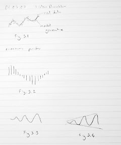
Sunday, March 11, 2007
IE 602 System Dynamics Lecture Notes 2007-03 - By Yaman Barlas
Subscribe to:
Post Comments (Atom)

No comments:
Post a Comment